前面幾篇文章提到 manifold learning,

只討論用於降維，沒有討論如何用於 learning.
什麼是 learning? No free lunch theorem told us need to (1) underline structure; (2) constraints to learn something from existing data.
underline structure => manifold hypothesis or kernel method, 如下式的 $H$ (function search space).
constraint => Occam razor principle, simpler is better than complex, smooth (underfit or just make) is better than curvy (overfit). => regularization, 如下式的 $R$

$\arg \min _{f \in \mathcal{H}} \hat{\mathcal{E}}(f, x, y)+\lambda R(f, x, y)$

上式可以化簡為：
$L(f, x, y)=L_{s u p}(y, f(x))+\gamma_{\mathcal{K}}\|f\|_{\mathcal{K}}^{2}+\gamma_{\mathcal{I}} R_{\mathcal{I}}(f)$
什麼是 Manifold learning? 就是考慮 manifold 的結構。問題是如何“考慮 manifold 的結構”？
一個簡潔優雅 learning 方法, 就是用 Laplacian operator 加在 loss function 做為 regularization term! 如上式的 $R_I(f)$ . 這個方法有物理意義 (minimum Laplacian = minimum energy, most smoothness, maximum variance?), 也容易計算 (Laplacian eigenvalue decomposition).
Manifold learning 是 machine learning 的拓展, 不是 deep learning.
Manifold learning 是 non-linear learning, i.e. dataset and/or decision boundary 是 non-linear.
Non-linear decision boundary (for supervised or semi-supervised learning) 很容易理解如下圖：
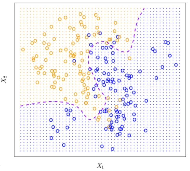
Non-linear dataset (for unsupervised/semi-supervised/supervised learning) 代表兩個 data 的平均不是另一個 data 如下圖的 swiss roll. 舉例兩個不同人臉，或是同一個人臉兩個不同角度的照片 (in pixel space) 平均值不會是另一個人臉。
Non-linear learning 分為兩類：(i) data independent, 例如 machine learning + kernel method, e.g. kernel-SVM. (ii) data dependent, 例如 manifold learning.
[@melas-kyriaziMathematicalFoundations2020] 把 kernel method 和 manifold learning 放在一個框架。 kernel method 即是 data independent regularization (kernel), manifold learning 即是 data dependent regularization 如下式。
注意，kernel method and manifold learning 是可以同時 apply 到一個 learning problem, 如下式。
Kernel method 是要解決 nonlinear decision boundary, 一般是用於 supervised learning. 精髓是把 low dimension data/space map 到 high dimension data/space 藉此把 data or decision boundary 變成 linear. 就是把下式的 $f(x) \to f(\phi(x))$ where $\phi(x)$ is the kernel function map low dimension $x$ to high dimension $\phi(x)$ .
Kernel method 可以 generalize to general learning problem: low dimension 複雜 function $f(x)$ 變成 high dimension 簡單 function $f(\phi(x))$ . 什麼是簡單 function? 就是 approximate the unknown function using linear combination in the Reduced Kernel Hilbert Space (RKHS). 因此可以用 $\|f\|^2_K$ for the regularization.
注意, conceptually, map low dimension data to high dimension RKHS 乍看之下變複雜，但是變成 linear problem 卻是變簡單。 Low dimension without kernel 需要用 piece-wise linear boundary to (over)-fit the data. High dimension linear boundary 反而簡化問題。所以 kernel method + corresponding regularization 更能 generalize to new data. 更重要是 kernel method exactly avoid the computation by using inner product computation at low dimension space!
因此 kernel method 可以視為 data independent extrinsic regularization.
Manifold learning 也是 nonlinear learning. Manifold hypothesis 是 high dimension data in pixel space 其實可以 map 到 low dimension manifold space. manifold learning from high dimension to low dimension，這和 kernel method from low dimension to high dimension 方法不同。
Manifold learning 是 data dependent intrinsic regularization.

舉個例子， PCA 就是簡單的 (linear) regularization term, ref. to paper for other regularization.
LLE, geodesic distance instead of Euclidean distance 可以代入成為 data dependent regularization term.

==> Key solution: kernel and manifold 都是用來 regulate (避免 overfit) the cost function! by impose the smoothness of the data (想一想 overfit curve) using a simpler structure. Kernel 是 extrinsic smoothness; manifold 是 intrinsic smoothness!! 學過 differential geometry 應該知道兩者差異！

Question:

What is kernel? Why use kernel (for nonlinearity?) or for distance?
- Kernel is a distance matrix, or a covariance matrix, or similarity matrix. 可以用 eigenvalue decomposition 得到 eigenvalues/eigenvectors. 可以忽略小的 eigenvalues/eigenvectors to 降維。用 Julia 做一個例子。
- Kernel is a distance function or similarity function given an anchor point, $x'$ . 兩者的形式類似但 distance function 是凹函數 (min when d=0)，similarity function 是凸函數 (max when d=0)。重點是利用 kernel function 為 base function 重組回 underlying function in the RKHS. 顯然 kernel function, $K(x, x')$ 應該用凸函數（i.e. similarity function) 為 base function.
- Distance function 有一個很大優點，就是 translation invariance and intuitive. 把 distance function convert to similarity function 一個簡單的方法：（1）-1* distance function + dc_offset; (2) put exp(-1*distance function) 或是加上 DC offset.
Why use kernel?
- 簡單說就是擴大 function search space $H$ (equation 1). 如果只 search linear space with regularization (e.g. SVM, PCA), 對於 nonlinear dataset (e.g. image) or nonlinear decision boundary performance 很差。 Linear space 可視為 kernel method 的特例。[@melas-kyriaziMathematicalFoundations2020]
- Kernel function with polynomial or radial kernel increase to higher or infinite dimension (linear space) to better deal with data nonlinearity, and more importantly can still compute efficiently.
Why the kernel is exp(-|distance|), 似乎沒有具象的物理意義?
- 滿足一些條件的 function (symmetry, positive definite, etc.) 就可以成為 kernel function, 保證存在對應的 RKHS 具有一些好的特性, e.g. inner product, linear combination.
Kernel 已經在處理 nonlinear data or decision boundary 問題，為什麼還需要 manifold learning. Kernel learning 和 manifold learning 有什麼關係？
- Kernel learning 比較像事有一些固定的招式 for data nonlinearity（polynomial, RBF with a few parameters to tune), 是原來 Euclidean search space 的推廣到 RKHS (high dimension) search space. 比較是 extrinsic view, 並不是從 data 本身特性出發。 Manifold learning 則是 explore data 本身的特性 (manifold or connection graph), 比較是 intrinsic view.
- 對於一些簡單的 manifold (e.g. circle, ball) kernel method 可能就有不錯的效果。但對於比較複雜的 manifold (e.g. swiss roll) manifold learning 比較有機會得到好的結果。 Kernel learning and manifold learning 都要有 constraints (smoothness/regularization) 避免 overfit.
- Kernel and manifold 都是用來 constraint the cost function by impose the smoothness of the data using a simpler structure. Kernel 是 extrinsic smoothness in RKHS space; manifold 是 intrinsic smoothness on the manifold!! 熟悉 differential geometry 應該知道兩者差異！
What is Laplacian? Why use Laplacian for both manifold learning and graph learning? 見下文。

Type	Kernel Learning	Manifold Learning
Geometry view	Extrinsic	Intrinsic
Space	RKHS	Data manifold
Operator	Kernel function	Laplacian operator
Data dependency	Indep. (e.g. kernel function)	Dependent (e.g. Laplacian)
Regularization	Explict. Tikhonov regul. ( $f_K$ )	Embedded in Laplacian
Supervised/semisupervised nonlinear learnign (decision boundary)	Widely used	this thesis?
Unsupervised nonlinear learning (e.g. dimension reduction)	Widely used (e.g. Kernel PCA)	Widely used (e.g. LE, LLE)
Smoothness/regularization	Smooth in RKHS	Smooth on manifold
Dimensionality	Low (feature space) to High (RKHS)	High (e.g. pixel space) to Low (manifold)
Nonlinearity Problem addressed?	Globally simpler manifold, e.g. circle, ball	Globally complicated manifold, but locally looks like Euclidean linear space

Key messages from the Harvard thesis [@melas-kyriaziMathematicalFoundations2020]

Manifold learning is a data dependent regularization with Laplacian operator
Laplacian operator are defined on both manifold and graph.
the Laplacian of the data graph converges to the Laplacian of the data manifold in the limit of infinite data.

Learning Algorithm & Loss Function

Math formulation of learning and regularization. Omit.

$\arg \min _{f \in \mathcal{H}} {\varepsilon}(f, x, y)+\lambda R(f, x, y)$

$\varepsilon(f) = \mathbb{E}[L(y, f(x)]$ , where $L(y, f(x))$ is the loss function, e.g. entropy loss, mean square loss, mean average loss.
是 regularization term. 分為
- Data independent, $R(f, x, y) = R(f)$ , e.g. L1 or L2 weight penalties.
- Data dependent regularization, $R(f, x, y)$ , e.g. manifold regularization, data augmentation regularization.

Specific issues:

How to define H to make optimization possible.
How to define $R$ to capture the essence complexity of a function.

如果 $f$ 是 vectors in R^d, both issues are easily solved. (1) solve the optimization problems over finite-dimensional Euclidean space. (2) use the vector norm $\|v\|$ (= x' x?) norm to capture the complexity of the function, developed by linear statistical learning.

現實當然不是 vectors, 我們用 Reproducing Kernel Hilbert Space (RKHS) 是 potentially-infinite-dimensional space that looks and feels like Euclidean space.

Hilbert space: a complete inner product space
Reproducing: additional smoothness property (the reproducing property).

同樣我們用 $\|.\|_K$ (= x' K x or exp(||x-y||) ) norm corresponding to the inner product of the RKHS to measure the complexity of functions.

Reproducing Kernel Hilbert Spaces (RKHS)

In summary, RKHS implies Tikhonov regularization?

Hilbert space V is a complete vector space 具有 inner product $\langle\cdot,\cdot\rangle$

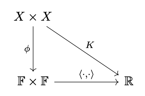
問題是 kernel 是什麼？如上圖是 feature map 的 inner product.

只要滿足 K 是 (1) symmetric; (2) semi-positive definite!
What is H_k ?

另外如果 K 是 translation invariance, i.e. K(x, y) = K(|x-y|), e.g. K(|x-y|) = exp(-|x-y|), 會有更多的特性，可以用 fourier transform. (eigenvector 就是不同的 fundmental frequencies).

最後的結論是 Kernel function $K: X \times X \to R$ is positive if and only if it may be written as $<\phi(.), \phi(.)>$ for some Hilbert space F and some map $\phi : X \to F$

This is not a new thing!

之前我們並不管在 feature domain 的 behavior, 直接計算 K. 此處花更多的篇幅討論 feature domain behavior,
- $K(x, y) = <\phi(x), \phi(y)>$ 是度量 x, y feature domain similarity.
- $d_K(x, y)^2 = |\phi(x)-\phi(y)|^2 = K(x, x) - 2 K(x, y) + K(y, y)$ 度量 x, y feature domain 的距離。

Tikhonov Regularization and the Representation Theory

$\arg \min _{f \in \mathcal{H}} {\varepsilon}(f, x, y)+\lambda R(f, x, y)$

Let R be the norm $\|f \|^2_K = K(f, f)$ to measure the complexity of the function. 這是一種 data independent regularization.

Graphic and (Riemannian) Manifold

本節 (Chapter 4 of the thesis) 主要論述 the geometry of graphs and Riemannian manifolds.

乍看之下， graph and manifold 是兩個非常不同的數學 objects. Graph 具有 combinatorial (discrete) properties, such as vertex, edge, etc. Manifold 具有 topological, geometric, differentiable properties, such as tangent, curvature, etc.

但更深入了解，graph 和 manifold 其實有關聯。其中的關鍵是 Laplacian operator 和對應的 spectral properties. 結論：graphs are discrete version of manifold and manifolds are continuous versions of graphs.

本文從 spectral properties of the Laplacian 了解 graphs and manifolds 的連結。

Laplacian and Smoothness

什麼是 smoothness on a graph?

Let $G = (V, E)$ be a connected, undirected graph with edge E and vertices V.
再來定義 function on G $f: V\to \mathbb{R}$ defined on vertices.

直觀上 f on a graph is smooth if its value at a node is similar to its value at each of the node's neighbors.

$\min \sum_{(i, j) \in E}(f(i)-f(j))^{2}$

上式是對稱的 quadratic form, 所以存在一個 symmetric matrix L such that

$\mathbf{f}^{T} \mathbf{L f}=\sum_{(i, j) \in E}(f(i)-f(j))^{2}$
where f = $(x(1), ..., x(n))$ for $n = |V|$

L 稱為 Laplacian of the graph G.

我們可以把 L 視為度量 smoothness of functions. L 愈小代表愈 smooth? Yes.
另一個 Laplacian 的特性時 translation invariance, 很容易從定義得出。
可以證明 $\mathbf{L} = D - A$ where $D_{ii} = deg(i)$ is a diagonal matrix of degrees of nodes. $A$ is the adjacent matrix. [@melas-kyriaziMathematicalFoundations2020]

Notation: Some texts work with normalized Laplacian L rather than the standard Laplacian L. The normalized Laplacian is given by $D^{-1 / 2} \mathbf{L} D^{-1 / 2} = I - D^{-1 / 2} A D^{-1 / 2}$ .

另外可以加上 weights, 定義 weighted graph, by the quadratic from:
$\mathbf{x}^{T} \mathbf{L} \mathbf{x}=\sum_{(i, j) \in E} w_{i j}(x(i)-x(j))^{2}$

我們看一些實際的例子：

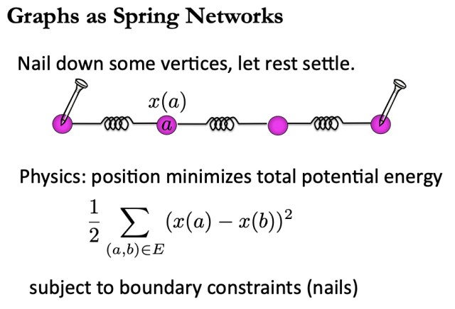
Minimize $\sum_{ij} w_{ij}(x_i - x_j)^2$ . 對應電路理論的最低功耗 (KVL) , $\sum_k V_k^2/R_k=\sum_k V_k^2 G_k$ , 或是 spring network 的最低勢能。

Graph Laplacian 特性

CYCLE GRAPH: 一個簡單的 graph 是 smooth cycle graph (or an infinite long path graph). The Laplacian L of a cycle graph G with n vertices is:
$latex \begin{aligned}
\mathbf{L} &=D-A=\left(\begin{array}{cccc}
2 & 0 & 0 & 0 \\
0 & \ddots & 0 & 0 \\
0 & 0 & 2 & 0 \\
0 & 0 & 0 & 2
\end{array}\right) \\
&=\left(\begin{array}{cccccc}
2 & -1 & 0 & 0 & 0 & -1 \\
-1 & 2 & -1 & 0 & 0 & 0 \\
0 & -1 & \ddots & \ddots & 0 & 0 \\
0 & 0 & \ddots & \ddots & -1 & 0 \\
0 & 0 & 0 & -1 & 2 & -1 \\
-1 & 0 & 0 & 0 & -1 & 2
\end{array}\right)
\end{aligned} $

這個 matrix L 有幾個非常有趣和重要的特性：

it's 2nd order difference equation. $\frac{\partial^{2} u}{\partial x^{2}} \approx-\frac{-u_{i+1}+2 u_{i}-u_{i-1}}{\delta x}$
Continuous Laplacian operator is 2nd order differentiation equation!
Eigenvalues are FFT of first row, impulse response! which is $2 - 2 \cos(2\pi k/n)$ , where $0 \le k \le n/2.$ Eigenvectors 是 harmonics, TBA.
以上結果可以推廣，稱為 Laplacian spectral graph theory.

下一步是 L matrix 的 eigenvalue decomposition, or spectrum analysis.

Laplacian Graph Spectral Theory

Assuming graph $G(V, E)$ with $n$ vertex and perform the eigenvalue decomposition of $\mathbf{L} = D - A$ ,

$\lambda_{n-1} \ge ...\ge\lambda_2\ge\lambda_1\ge\lambda_0=0$
因為 x=(1,1,…,1)' 對應 $Lx=\lambda_0 x$ , and $\lambda_0=0$ .
$\lambda_1$ 對應最少 cut 的 graph partition. 所以 $\lambda_1=0$ 代表 graph 有不連通的 subgraphs, $G_1$ and $G_2$
因為 x = (1, 1, .. -1, -1) 對應 $Lx=\lambda_1 x$ , and $\lambda_1=0$ . Note L 的左上 block 是 $G_1$ , 右上 block 是 $G_2$ .
以此類推，如果有三個不聯通的 subgroups, x = (1, 1,.. ,-1, -1,.., 1,1,..) 對應 $Lx=\lambda_2 x$ , and $\lambda_2=0$ .

[@cookMeasuringConnectivity2016] 有一些例子 provides “continuous measure" of graph connection using eigenvalue.

最大的 eigenvalue $\lambda_{n-1} \le n$ . 等號成立是 fully connected graph, 如下圖。類似 impulse noise 的 FFT 是 white spectrum!

A = [4 -1 -1 -1 -1; -1 4 -1 -1 -1 ; -1 -1 4 -1 -1 ; -1 -1 -1 4 -1 ; -1 -1 -1 -1 4]
eigvals(A)

5×5 Array{Int64,2}:
  4  -1  -1  -1  -1
 -1   4  -1  -1  -1
 -1  -1   4  -1  -1
 -1  -1  -1   4  -1
 -1  -1  -1  -1   4

5-element Array{Float64,1}:
 0.0
 5.0
 5.0
 5.0
 5.0

其他的 graph connection 對應的 eigenvalues 都小於 n. 愈多的 edges 對應大的 eigenvalues.
另一個完全相反的 graph of star, eigenvalues 非常有趣。最大 eigenvalue = n, 的對應 central vertex，基本是 fully connected. 其他 vertex 只有一個 edge, 對應 eigenvalue = 1.

B = [5 -1 -1 -1 -1 -1 ; -1 1 0 0 0 0 ;  -1 0 1 0 0 0 ; -1 0 0 1 0 0 ; -1 0 0 0 1 0; -1 0 0 0 0 1]
eigvals(B)

6×6 Array{Int64,2}:
  5  -1  -1  -1  -1  -1
 -1   1   0   0   0   0
 -1   0   1   0   0   0
 -1   0   0   1   0   0
 -1   0   0   0   1   0
 -1   0   0   0   0   1

julia> eigvals(B)
6-element Array{Float64,1}:
  0.0
  1.0                  
  1.0                  
  1.0                  
  1.0   
  6.0

What is the solution? Spectral analysis of $L$ ?

Smoothness on a Manifold

Let $(M, g)$ be a Riemannian manifold of dimension n. M 是 smooth manifold (local 看起來像 Euclidean space), g 是 metric assigned to $x \in M$ an inner product $\langle\cdot,\cdot\rangle_{g_x}$ on the tangent space $T_x M$ at $x$ .

如何度量 manifold smoothness? 同樣用 $\|\nabla f\|^2$ . 可以用 Dirichlet energy denoted by $E[f] = \frac{1}{2} \int_M \|\nabla f(x)\|^2 dx$

The functional derivative of Dirichlet energy, i.e. minimum Dirichlet energy, 就是 Laplacian operator, $\Delta f = -\lambda f$ .

For Euclidean space
$\Delta f=-\frac{\partial^{2} f}{\partial x^{2}}-\frac{\partial^{2} f}{\partial y^{2}}-\frac{\partial^{2} f}{\partial z^{2}}$

For general manifold,
$\Delta=-\frac{1}{\sqrt{|\operatorname{det} g|}} \sum_{i, j=1}^{n}\left(g^{i j} \sqrt{|\operatorname{det} g|} \frac{\partial}{\partial x_{j}}\right)$

~~而且神奇的 $\|\nabla f\|^2 \approx f\nabla \cdot \nabla f \approx \nabla^2 f$ .~~

這對於一些 non-euclidean (i.e. manifold) test dataset (e.g. Swiss roll) 或是 real life data (e.g. image), 當然會有很大的差距。

另外像 LLE (local linear embedded) 就比較有 manifold 的概念。只看 local 特性，仍然是 Euclidean space, 但是 globally 可以是 non-euclidean manifold. 不過也沒有 explore manifold 的特性。

另外有 Laplacian eigenvector/eigenvalue, ISOMap, 比較有利用 manifold, 主要是找出 nearest neighbours.

此時多了兩個 concepts: kernel! and Lapacian! So What is the concepts???????????????????? coming from????

Kernel can be regarded as duality of distance!!!!!!!!1
So what is Laplacing????