Math AI: Maximum Likelihood Estimation (MLE) Evolve To EM Algorithm For Incomplete/Hidden Data To Variational Bayesian Inference

Major Reference

[@poczosCllusteringEM2015]
[@matasExpectationMaximization2018] good reference
[@choyExpectationMaximization2017]
[@tzikasVariationalApproximation2008] excellent introductory paper

Maximum Likelihood Estimation 和應用

Maximum likelihood estimation (MLE) 最大概似估計是一種估計模型參數的方法。適用時機在於手邊有模型，但是模型參數有無限多種，透過真實觀察到的樣本資訊，想辦法導出最有可能產生這些樣本結果的模型參數，也就是挑選使其概似性(Likelihood)最高的一組模型參數，這系列找參數的過程稱為最大概似估計法。

Bernoulli distribution：投擲硬幣正面的機率 $\theta$ , 反面的機率 $1-\theta$ . 連續投擲的正面/反面的次數分別是 H/T. Likelihood function 為

$f(\theta, H, T)=\theta^{H}(1-\theta)^{T}$

MLE 在無限個 $\theta$ 中，找到一個使概似性最大的 $\theta$ , i.e. $\widehat{\theta}_{\mathrm{MLE}} =\arg \max _{\theta} {\theta^{H}(1-\theta)^{T}}$

只要 likelihood function 一次微分，可以得到

$\widehat{\theta}_{M L E}=\frac{H}{T+H}$

就是平均值，推導出來的模型參數符合直覺。

Normal distribution：假設 mean unknown, variance known, 我們可以用 maximum log-likelihood function

$\underset{\mu}{\operatorname{argmax}} f\left(x_{1}, \ldots, x_{n}\right) \Rightarrow \underset{\mu}{\operatorname{argmax}} \log f\left(x_{1}, \ldots, x_{n}\right)$

$latex \begin{aligned}
&\frac{\mathrm{d}}{d \mu}\left(\sum_{i=1}^{n}-\frac{\left(x_{i}-\mu\right)^{2}}{2 \sigma^{2}}\right)=\sum_{\mathrm{i}=1}^{\mathrm{n}} \frac{\left(x_{i}-\hat{\mu}\right)}{\sigma^{2}}=\sum_{i=1}^{n} x_{i}-n \hat{\mathrm{u}}=0 \\
&\hat{\mu}=\overline{\mathrm{X}}=\frac{\sum_{i=1}^{n} x_{i}}{n}
\end{aligned} $

微分的結果告訴我們，樣本的平均值，其實就是母體平均值 $\mu$ 最好的估計！又是一個相當符合直覺的答案，似乎 MLE 只是用來驗證直覺的工具。

這是一個錯覺，常見的 distribution (e.g. Bernoulli, normal distribution) 都是 exponential families. 可以證明 maximum log-likelihood functions of exponential families 都是 concave function, 沒有 local minimum. 非常容易用數值方法找到最佳解，而且大多有 analytical solution.

但只要 distribution function 更複雜一點，例如兩個 normal distribution weighted sum to 1, MLE 就非常難解。這是 EM algorithm 為什麼非常有用。

Maximum Likelihood Estimation (MLE) vs. EM

EM seems to be a special case for MLE?
- Yes! If the problem can be formulated as MLE of incomplete/hidden data. Then EM algorithm 的 E-step is guessing incomplete/hidden data; M-step 就對應 MLE with some modification (見本文後段)。
Sometimes MLE is very hard to solve because of too many parameters to estimation (mean, variance, initial distribution in GMM; or initial distribution, transition probability, emission probability in HMM); or missing data or missing label!!
- Too many parameters can be seen as incomplete/hidden data. see the following GMM example. It can be regards as missing label.
In the above case, EM is a specialized MLE with iterative approach to solve the MLE.
- Yes. Specifically, the M step is MLE.
EM ~~ iterative MLE (maybe local minimum)
EM is more general than MLE because it can apply to parameters and missing data?
- The same thing, unknown parameters can be regarded as missing information/data. In the M step, we guess the missing data. In the E step, we use MLE to compute it, and so on.

Toy Example [@matasExpectationMaximization2018]

前提摘要

一個簡單例子觀察 temperature and amount of snow (溫度和雪量, both are binary input) 的 joint probability depending on two "scalar factors" $a$ and $b$ as $p(t, s | a, b)$

	$s_0$	$s_1$
$t_0$	$a$	$5a$
$t_1$	$3b$	$b$

注意 $a$ and $b$ are parameters, 不是 conditional probability.
另外因為機率和為 1 做為一個 constraint: $6a + 4b = 1$

問題一: MLE

一個 ski-center 觀察 $N$ 天的溫度和雪量得到以下的統計， $N_{ij} \in \mathbf{I}$ , 如何估計 $a$ and $b$ ?

	$s_0$	$s_1$
$t_0$	$N_{00}$	$N_{01}$
$t_1$	$N_{10}$	$N_{11}$

Likelihood function (就是 joint pdf of $N$ repeat experiments)

$P(\mathcal{T} \mid a, b)= C a^{N_{00}}(5 a)^{N_{01}}(3 b)^{N_{10}}(b)^{N_{11}}$

where $C = (\Sigma N_{ij})! / \Pi (N_{ij}!)$ 是 MLE 無關的常數

問題改成 maximum log-likelihood with constraint and $C' = \ln C$

$L(a, b, \lambda) = C' + N_{00} \ln a+N_{01} \ln 5 a+N_{10} \ln 3 b+N_{11} \ln b+\lambda(6 a+4 b-1)$

$latex \begin{gathered}
\frac{\partial L}{\partial a}=N_{00} \frac{1}{a}+N_{01} \frac{1}{a}+6 \lambda=0 \\
\frac{\partial L}{\partial b}=N_{10} \frac{1}{b}+N_{11} \frac{1}{b}+4 \lambda=0 \\
\frac{\partial L}{\partial \lambda}=6 a+4 b – 1 = 0
\end{gathered} $

上述方程式的解為
$a=\frac{N_{00}+N_{01}}{6 N} \quad b=\frac{N_{10}+N_{11}}{4 N} \quad \lambda = -(N_{00}+N_{01}+N_{10}+N_{11})=-N$

結果很直觀。其實就是利用大數法則： $a\cdot N \sim N_{00}; 5a\cdot N\sim N_{01}; 3b\cdot N\sim N_{10}; b\cdot N\sim N_{11}$
再來大數法則 (a+5a)N~N00+N01; (3b+b)N~N10+N11 => a = .. ; b = …

問題二 incomplete/hidden Data

假設我們無法觀察到完整的"溫度和雪量“；而是“溫度或雪量”，有時“溫度”，有時“雪量”，但不是同時。對應的不是 joint pdf, 而是 marginal pdf 如下：

觀察如下：

The Lagrangian (log-likelihood with constraint)

$L(a, b, \lambda)=T_{0} \ln 6 a+T_{1} \ln 4 b+S_{0} \ln (a+3 b)+S_{1} \ln (5 a+b)+\lambda(6 a+4 b-1)$

此時的方程式比起之前複雜的多，不一定有 close-form solution:

$latex \begin{gathered}
\frac{\partial L}{\partial a}=\frac{T_{0}}{a}+\frac{S_{0}}{a+3 b}+\frac{5 S_{1}}{5 a+b}+6 \lambda=0 \\
\frac{\partial L}{\partial b}=\frac{T_{1}}{b}+\frac{3 S_{0}}{a+3 b}+\frac{S_{1}}{5 a+b}+4 \lambda=0 \\
6 a+4 b=1
\end{gathered} $

如果用大數法則：

$6a \cdot(T_0+T_1) \sim T0; \, 4b\cdot(T_0+T_1) \sim T_1$
$(a+3b) \cdot (S_0+S_1)\sim S_0; \, (5a+b)\cdot(S_0+S_1) \sim S_1$
注意不論 1. or 2. 都滿足 $6a+4b = 1$ constraint, 可以用來估計 $a$ and $b$ .
問題是我們要用那一組 $(a, b)$ ? 單獨用一組都會損失一些 information, 應該要 combine 1 and 2 的 information, how?

思路一 平均 (a, b) from 1 and 2. 但這不是好的策略，因為平均 (a,b) 不一定滿足 constraint. 在這個 case 因為 linear constraint, 所以平均 (a,b) 仍然滿足 constraint. 但對於更複雜 constraint, 平均並非好的方法。

更重要的是平均並無法代表 maximum likelihood in the above equation. 我們的目標是 maximum likelihood, 平均 (a, b) 完全無法保證會得到更好的 likelihood value!

或者把 (a,b) from 1 or 2 代入上述 likelihood function 取大值。顯然這也不是最好的策略。因為一半的資訊被捨棄了。

思路二 比較好的方法是想辦法用迭代法解微分後的 Lagrange multiplier 聯立方程式。 (a, b) from 1. or 2. 只作為 initial solution, 想辦法從聯立方程式找出 iterative formula. 這似乎是對的方向，問題是 Lagrange multiplier optimization 是解聯立(level 1)微分方程式。不一定有 close form as in this example. 同時也無法保證收斂。另外如何找出 iterative formula 似乎是 case-by-case, 沒有一致的方式。
=> iterative solution is one of the key, but NOT on Lagrange multiplier (level 1)

思路三 既然是 missing data, 我們是否可以假設 $(a, b) \to$ fill missing data $\to$ update $(a, b) \to$ update missing data $\cdots$ 具體做法
$N_{00} = T_0 \cdot \frac{1}{6} + S_0 \cdot \frac{a}{a+3b}$
$N_{01} = T_0 \cdot \frac{5}{6} + S_1 \cdot \frac{5a}{5a+b}$
$N_{10} = T_1 \cdot \frac{3}{4} + S_0 \cdot \frac{3b}{a+3b}$
$N_{11} = T_1 \cdot \frac{1}{4} + S_1 \cdot \frac{b}{5a+b}$

有了 $N_{00},N_{01},N_{10},N_{11}$ 可以重新估計 $(a, b)$ using joint pdf

$a'=\frac{N_{00}+N_{01}}{6 N} \quad b'=\frac{N_{10}+N_{11}}{4 N}$

Q: 如何證明這個方法是最佳或是對應 complete data MLE or incomplete/hidden data MLE? 甚至會收斂？

EM algorithm 邏輯

前提摘要

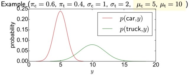
GMM 特例：Estimate Means of Two Gaussian Distributions (known variance and ratio; unknown means)

We measure lengths of vehicles. The observation space is two-dimensional, with $x$ capturing vehicle type (binary) and $y$ capturing length (Gaussian).

$p(x, y)$ $x\in$ {car, truck}, $y \in \mathbb{R}$

$p(\text {car}, y)=\pi_{\mathrm{c}} \mathcal{N}\left(y \mid \mu_{\mathrm{c}}, \sigma_{\mathrm{c}}=1\right)=\kappa_{\mathrm{c}} \exp \left\{-\frac{1}{2}\left(y-\mu_{\mathrm{c}}\right)^{2}\right\},\left(\kappa_{\mathrm{c}}=\frac{\pi_{\mathrm{c}}}{\sqrt{2 \pi}}\right)$

$p(\text {truck,} y)=\pi_{\mathrm{t}} \mathcal{N}\left(y \mid \mu_{\mathrm{t}}, \sigma_{\mathrm{t}}=2\right)=\kappa_{\mathrm{t}} \exp \left\{-\frac{1}{8}\left(y-\mu_{\mathrm{t}}\right)^{2}\right\},\left(\kappa_{\mathrm{t}}=\frac{\pi_{\mathrm{t}}}{\sqrt{8 \pi}}\right)$

where $\pi_c + \pi_t = 1$

問題三 Complete Data (Easy case)

$T=\{\underbrace{\left(\operatorname{car}, y_{1}^{(c)}\right),\left(\operatorname{car}, y_{2}^{(c)}\right), \ldots,\left(\operatorname{car}, y_{C}^{(c)}\right)}_{C \text { car observations }}, \underbrace{\left(\text {truck}, y_{1}^{(\mathrm{t})}\right),\left(\text {truck}, y_{2}^{(\mathrm{t})}\right), \ldots,\left(\text {truck}, y_{T}^{(\mathrm{t})}\right)}_{T \text { truck observations }}\}$

Log-likelihood

$\ell(\mathcal{T})=\sum_{i=1}^{N} \ln p\left(x_{i}, y_{i} \mid \mu_{\mathrm{c}}, \mu_{\mathrm{t}}\right)=C \ln \kappa_{\mathrm{c}}-\frac{1}{2} \sum_{i=1}^{C}\left(y_{i}^{(c)}-\mu_{\mathrm{c}}\right)^{2}+T \ln \kappa_{\mathrm{t}}-\frac{1}{8} \sum_{i=1}^{T}\left(y_{i}^{(\mathrm{t})}-\mu_{\mathrm{t}}\right)^{2}$

很容易用 MLE 估計 $\mu_1, \mu_2$

$\frac{\partial \ell(\mathcal{T})}{\partial \mu_{\mathrm{c}}}=\sum_{i=1}^{C}\left(y_{i}^{(\mathrm{c})}-\mu_{\mathrm{c}}\right)=0 \quad \Rightarrow \quad \mu_{\mathrm{c}}=\frac{1}{C} \sum_{i=1}^{C} y_{i}^{(c)}$

$\frac{\partial \ell(\mathcal{T})}{\partial \mu_{\mathrm{t}}}=\frac{1}{4} \sum_{i=1}^{T}\left(y_{i}^{(\mathrm{t})}-\mu_{\mathrm{t}}\right)=0 \quad \Rightarrow \quad \mu_{\mathrm{t}}=\frac{1}{T} \sum_{i=1}^{T} y_{i}^{(\mathrm{t})}$

直觀上很容易理解。如果 observations 已經分組，求 mean 只要做 sample 的平均即可。

以這個例子，ratio $\pi_c, \pi_t$ 不論已知或未知，都不影響結果。

問題四 incomplete/hidden Data

$latex \mathcal{T}=\{\left(\operatorname{car}, y_{1}^{(c)}\right), \ldots,\left(\operatorname{car}, y_{C}^{(c)}\right),\left(\text {truck}, y_{1}^{(\mathrm{t})}\right), \ldots,\left(\text {truck}, y_{T}^{(\mathrm{t})}\right), \underbrace{\left(\bullet, y_{1}^{\bullet}\right), \ldots,\left(\bullet, y_{M}^{\bullet}\right)}_{\begin{array}{l}
\text { data with uknown } \\
\text { vehicle type }
\end{array}}\} $

$p\left(y^{\bullet}\right)=p\left(\text {car}, y^{\bullet}\right)+p\left(\text {truck}, y^{\bullet}\right)$

Log-likelihood

$latex \ell(\mathcal{T})=\sum_{i=1}^{N} \ln p\left(x_{i}, y_{i} \mid \mu_{c}, \mu_{\mathrm{t}}\right)=\overbrace{C \ln \kappa_{\mathrm{c}}-\frac{1}{2} \sum_{i=1}^{C}\left(y_{i}^{(c)}-\mu_{\mathrm{c}}\right)^{2}+T \ln \kappa_{\mathrm{t}}-\frac{1}{8} \sum_{i=1}^{T}\left(y_{i}^{(\mathrm{t})}-\mu_{\mathrm{t}}\right)^{2}}^{\text {same term as before }} \\
+\sum_{i=1}^{M} \ln \left(\kappa_{\mathrm{c}} \exp \left\{-\frac{1}{2}\left(y_{i}^{\bullet}-\mu_{\mathrm{c}}\right)^{2}\right\}+\kappa_{\mathrm{t}} \exp \left\{-\frac{1}{8}\left(y_{i}^{\bullet}-\mu_{\mathrm{t}}\right)^{2}\right\}\right) $

不用微分也知道非常難解 MLE. 我們必須用另外的方法，就是 EM 算法。
不過我們還是微分一下，得到更多的 insights.

$latex \begin{aligned}
0=\frac{\partial \ell(\mathcal{T})}{\partial \mu_{\mathrm{c}}} &=\sum_{i=1}^{C}\left(y_{\mathrm{c}}^{(\mathrm{c})}-\mu_{\mathrm{c}}\right) \\
&+ \sum_{i=1}^{M} \overbrace{\frac{\kappa_{\mathrm{c}} \exp \left\{-\frac{1}{2}\left(y_{i}^{\bullet}-\mu_{\mathrm{c}}\right)^{2}\right\}}{\kappa_{\mathrm{c}} \exp \left\{-\frac{1}{2}\left(y_{i}^{\bullet}-\mu_{\mathrm{c}}\right)^{2}\right\}+\kappa_{\mathrm{t}} \exp \left\{-\frac{1}{8}\left(y_{i}^{\bullet}-\mu_{\mathrm{t}}\right)^{2}\right\}}}^{p\left(\operatorname{car} \mid y_{i}^{\bullet}, \mu_{\mathrm{c}}, \mu_{\mathrm{t}}\right)}\left(y_{i}^{\bullet}-\mu_{\mathrm{c}}\right)
\end{aligned} $

$0=4 \frac{\partial \ell(\mathcal{T})}{\partial \mu_{\mathrm{t}}}=\sum_{i=1}^{T}\left(y_{i}^{(\mathrm{t})}-\mu_{\mathrm{t}}\right)+\sum_{i=1}^{M} p\left(\text {truck} \mid y_{i}^{\bullet}, \mu_{\mathrm{c}}, \mu_{\mathrm{t}}\right)\left(y_{i}^{\bullet}-\mu_{\mathrm{t}}\right)$

上兩式非常有物理意義。基本是 easy case 的延伸：已知分類的平均值，加上未知分類的機率平均值。一個簡單的方法是只取前面已知的部分平均，不過這不是最佳，因為丟失部分的資訊。

Missing Values, EM Approach

重新 summarize optimality conditions

$\sum_{i=1}^{C}\left(y_{i}^{(c)}-\mu_{c}\right)+\sum_{i=1}^{M} p\left(\operatorname{car} \mid y_{i}^{\bullet}, \mu_{c}, \mu_{\mathrm{t}}\right)\left(y_{i}^{\bullet}-\mu_{\mathrm{c}}\right)=0$

$\sum_{i=1}^{T}\left(y_{i}^{(\mathrm{t})}-\mu_{\mathrm{t}}\right)+\sum_{i=1}^{M} p\left(\text {truck } \mid y_{i}^{\bullet}, \mu_{\mathrm{c}}, \mu_{\mathrm{t}}\right)\left(y_{i}^{\bullet}-\mu_{\mathrm{t}}\right)=0$

如果 $p(\text {truck} \mid y_{i}^{\bullet}, \mu_c, \mu_t)$ 和 $p(\text {car} \mid y_{i}^{\bullet}, \mu_c, \mu_t)$ 已知，上式非常容易解 $\mu_c$ and $\mu_t$ 。實際這是一個雞生蛋、蛋生雞的問題，因為這兩個機率又和 $\mu_c$ and $\mu_t$ 相關。

EM algorithm 剛好用來打破這個迴圈。

Let $z_i \,(i=1, 2, \cdots, M), z_i \in \text{\{car, truck\}}$ denote the missing data. Define $q\left(z_{i}\right)=p\left(z_{i} \mid y_{i}^{\bullet}, \mu_{\mathrm{c}}, \mu_{\mathrm{t}}\right)$
上述 optimality equations 可以得到

$\mu_{\mathrm{c}}=\frac{\sum_{i=1}^{C} y_{i}^{(\mathrm{c})}+\sum_{i=1}^{M} q\left(z_{i}=\mathrm{car}\right) y_{i}^{\bullet}}{C+\sum_{i=1}^{M} q\left(z_{i}=\mathrm{car}\right)}$

$\mu_{\mathrm{t}}=\frac{\sum_{i=1}^{T} y_{i}^{(\mathrm{t})}+\sum_{i=1}^{M} q\left(z_{i}=\text { truck }\right) y_{i}^{\bullet}}{T+\sum_{i=1}^{M} q\left(z_{i}=\text { truck }\right)}$

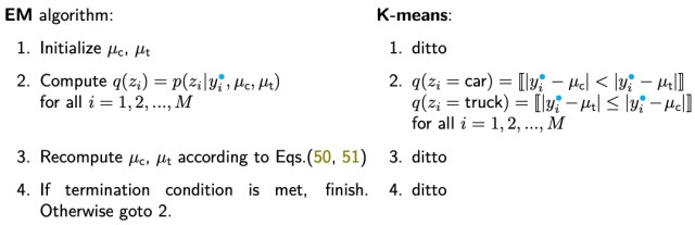
EM Algorithm 可以用以下四步驟表示

Initialize $\mu_c$ , $\mu_t$
Compute $q\left(z_{i}\right)=p\left(z_{i} \mid y_{i}^{\bullet}, \mu_{\mathrm{c}}, \mu_{\mathrm{t}}\right)$ for $i = 1, 2, \cdots, M$
Recompute $\mu_c$ , $\mu_t$ according to the above equations.
If termination condition is met, finish. Otherwise, goto 2.

上述步驟 2 稱為 Expectation (E) Step, 步驟 3 稱為 Maximization (M) Step. 統稱為 EM algorithm.

Q. Why Step 2 稱為 Expectation? not clear. Maximization 比較容易理解，因為 optimality condition 就是 maximization (微分為 0).

In summary, EM algorithm 的一個關鍵點是：讓 incomplete/hidden data 變成 complete (Expectation?). 有了完整的 data, 就容易用 MLE 找到 maximal likelihood estimation ( $\mu_c$ and $\mu_t$ in this case).

Clustering: Soft Assignment Vs. Hard Assignment (K-means)

EM Algorithm Derivation

EM algorithm 如果只是 heuristic algorithm, 可能有用度減半。這裡討論數學上的 justification. 先定義 terminologies

$\mathbf{o}$ : all observed values
$\mathbf{z}$ : all unobserved values (i.e. hidden variable)
$\mathbf{\theta}$ : model parameters to be estimated

目標：Find $\theta^*$ using the Maximum Likelihood approach

$\boldsymbol{\theta}^{*}=\underset{\boldsymbol{\theta}}{\operatorname{argmax}} \ell(\boldsymbol{\theta})=\underset{\boldsymbol{\theta}}{\operatorname{argmax}} \ln p(\mathbf{o} \mid \boldsymbol{\theta})$

思路：假設解下列完整 data 很容易解 (例如上面的 exmple xx and xx)

$\underset{\boldsymbol{\theta}}{\operatorname{argmax}} \ln p(\mathbf{o}, \mathbf{z} \mid \boldsymbol{\theta})$

我們的想法是把上上式改寫成上式，再加以優化
$latex \begin{aligned}
\ln p(\mathbf{o} \mid \boldsymbol{\theta}) &=\ln \sum_{\mathbf{z}} p(\mathbf{o}, \mathbf{z} \mid \boldsymbol{\theta}) \\
&=\ln \sum_{\mathbf{z}} q(\mathbf{z}) \frac{p(\mathbf{o}, \mathbf{z} \mid \boldsymbol{\theta})}{q(\mathbf{z})}
\end{aligned} $

這裡引入 $q(\mathbf{z})$ distribution with $\sum_{\mathbf{z}} q(\mathbf{z})=1$ . 上式利用 Jensen's inequality 可以導出
$\geq \sum_{\mathbf{z}} q(\mathbf{z}) \ln \frac{p(\mathbf{o}, \mathbf{z} \mid \boldsymbol{\theta})}{q(\mathbf{z})}$

Log-Likelihood with Hidden Variable Lower Bound

我們定義 $\ln p(\mathbf{o} \mid \boldsymbol{\theta})$ 的 lower bound $\mathcal{L}(q, \boldsymbol{\theta})$ , for any distribution $q$ .

$\mathcal{L}(q, \boldsymbol{\theta})=\sum_{\mathbf{z}} q(\mathbf{z}) \ln \frac{p(\mathbf{o}, \mathbf{z} \mid \boldsymbol{\theta})}{q(\mathbf{z})}$

這已經非常接近思路！

Maximizing $\mathcal{L}(q, \boldsymbol{\theta})$ by choosing $q(z)$ 就可以 push the log likelihood $\ln p(\mathbf{o} \mid \boldsymbol{\theta})$ upwards.

反過來我們可以計算和 lower bound 之間的 gap.

$latex \begin{aligned}
\ln p(\mathbf{o} \mid \boldsymbol{\theta})-\mathcal{L}(q, \boldsymbol{\theta}) &=\ln p(\mathbf{o} \mid \boldsymbol{\theta})-\sum_{\mathbf{z}} q(\mathbf{z}) \ln \frac{p(\mathbf{o}, \mathbf{z} \mid \boldsymbol{\theta})}{q(\mathbf{z})} \\
&=\ln p(\mathbf{o} \mid \boldsymbol{\theta})-\sum_{\mathbf{z}} q(\mathbf{z})\{\ln \underbrace{p(\mathbf{o}, \mathbf{z} \mid \boldsymbol{\theta})}_{p(\mathbf{z} \mid \mathbf{o}, \boldsymbol{\theta}) p(\mathbf{o} \mid \boldsymbol{\theta})}-\ln q(\mathbf{z})\} \\
&=\ln p(\mathbf{o} \mid \boldsymbol{\theta})-\sum_{\mathbf{z}} q(\mathbf{z})\{\ln p(\mathbf{z} \mid \mathbf{o}, \boldsymbol{\theta})+\ln p(\mathbf{o} \mid \boldsymbol{\theta})-\ln q(\mathbf{z})\} \\
&=\ln p(\mathbf{o} \mid \boldsymbol{\theta})-\underbrace{\sum_{\mathbf{z}} q(\mathbf{z})}_{1} \ln p(\mathbf{o} \mid \boldsymbol{\theta})-\sum_{\mathbf{z}} q(\mathbf{z})\{\ln p(\mathbf{z} \mid \mathbf{o}, \boldsymbol{\theta})-\ln q(\mathbf{z})\} \\
&=-\sum_{\mathbf{z}} q(\mathbf{z}) \ln \frac{p(\mathbf{z} \mid \mathbf{o}, \boldsymbol{\theta})}{q(\mathbf{z})} \\
&= D_{\mathrm{KL}}(q(\mathbf{z}) \| p(\mathbf{z} \mid \mathbf{o}, \boldsymbol{\theta}) ) \ge 0
\end{aligned} $

這個 gap 就是 KL divergence between $q(\mathbf{z})$ and $p(\mathbf{z} \mid \mathbf{o}, \boldsymbol{\theta})$ , 永遠大於 0.
如果能找到 $q(\mathbf{z}) = p(\mathbf{z} \mid \mathbf{o}, \boldsymbol{\theta})$ ，就可以讓 gap 變成 0.

EM Algorithm Push the Lower Bound Upwards

Log likelihood function 可以分為兩個部分： lower bound + gap
$\ln p(\mathbf{o} \mid \boldsymbol{\theta})=\mathcal{L}(q, \boldsymbol{\theta})+D_{\mathrm{KL}}(q \| p)$

從 Jensen's inequality 得到 $\mathcal{L}(q, \boldsymbol{\theta})$ 是 lower bound. 同樣從 KL divergence $\ge$ 0 再度驗證。

如果 $q(\mathbf{z}) = p(\mathbf{z} \mid \mathbf{o}, \boldsymbol{\theta})$ , the bound is tight.

Example 1: Hidden variable $z$ does NOT provide any information of $o$

假設 $\mathbf{o}$ 和 $\mathbf{z}$ 完全無關， $p(\mathbf{z} \mid \mathbf{o}, \boldsymbol{\theta}) = p(\mathbf{z} \mid \boldsymbol{\theta})$ . We can make $q(\mathbf{z}) = p(\mathbf{z} \mid \boldsymbol{\theta})$
such that $D_{\mathrm{KL}}(q(\mathbf{z}) \| p(\mathbf{z} \mid \mathbf{o}, \boldsymbol{\theta})) = 0$ , 也就是 gap = 0.

Lower bound 就變成原來的 log-likelihood function.
$latex \begin{aligned}
\mathcal{L}(q, \boldsymbol{\theta}) &= \sum_{\mathbf{z}} q(\mathbf{z}) \ln \frac{p(\mathbf{o}, \mathbf{z} \mid \boldsymbol{\theta})}{q(\mathbf{z})}\\
&= \sum_{\mathbf{z}} q(\mathbf{z}) \ln \frac{p(\mathbf{o} \mid \boldsymbol{\theta}) p(\mathbf{z} \mid \boldsymbol{\theta})}{q(\mathbf{z})} \\
&= \sum_{\mathbf{z}} q(\mathbf{z}) \ln p(\mathbf{o} \mid \boldsymbol{\theta})\\
&= \ln p(\mathbf{o} \mid \boldsymbol{\theta})
\end{aligned} $

Example 2: $q(\mathbf{z}) = p(\mathbf{z} \mid \mathbf{o}, \boldsymbol{\theta})$

$latex \begin{aligned}
\mathcal{L}(q, \boldsymbol{\theta}) &= \sum_{\mathbf{z}} q(\mathbf{z}) \ln \frac{p(\mathbf{o}, \mathbf{z} \mid \boldsymbol{\theta})}{q(\mathbf{z})}\\
&= \sum_{\mathbf{z}} q(\mathbf{z}) \ln \frac{p(\mathbf{z} \mid \mathbf{o}, \boldsymbol{\theta}) p(\mathbf{o} \mid \boldsymbol{\theta})}{q(\mathbf{z})} \\
&= \sum_{\mathbf{z}} q(\mathbf{z}) \ln p(\mathbf{o} \mid \boldsymbol{\theta})\\
&= \ln p(\mathbf{o} \mid \boldsymbol{\theta})
\end{aligned} $

What is the mutual information of $o$ and $z$ in this case?

EM 具體步驟

Lower bound $\mathcal{L}(q, \boldsymbol{\theta})$

$\mathcal{L}(q, \boldsymbol{\theta})=\sum_{\mathbf{z}} q(\mathbf{z}) \ln \frac{p(\mathbf{o}, \mathbf{z} \mid \boldsymbol{\theta})}{q(\mathbf{z})}$

Lower bound 其實可以視為 MLE of complete data，對應 EM algorithm 的 M step.
Gap 可以視為從 observables 推論出 unobservables, i.e. incomplete/hidden data, 對應 EM algorithm 的 E step.

Lower bound 包含兩個部分： (1) log-likelihood of complete data (both $o$ and $z$ ) MLE for $\theta$ estimation; (2) $q$ distribution.

這兩個部分剛好對應 EM algorithm 的 E-step and M-step.

Initialize $\boldsymbol{\theta}=\boldsymbol{\theta}^{(0)}$
E-step (Expectation): $q^{(t+1)}=\underset{q}{\operatorname{argmax}} \mathcal{L}\left(q, \boldsymbol{\theta}^{(t)}\right)$
M-step (Maximization): $\boldsymbol{\theta}^{(t+1)}=\underset{\boldsymbol{\theta}}{\operatorname{argmax}} \mathcal{L}\left(q^{(t+1)}, \boldsymbol{\theta}\right)$

M-step: $q^{(t+1)}$ is fixed

我們先看 M-step, 因為這和 MLE estimate $\theta$ 非常相似。

$\theta^{(t+1)}=\underset{\theta}{\operatorname{argmax}} \mathcal{L}\left(q^{(t+1)}, \theta\right)$

$latex \begin{aligned}
\mathcal{L}\left(q^{(t+1)}, \boldsymbol{\theta}\right) &=\sum_{\mathbf{z}} q^{(t+1)}(\mathbf{z}) \ln \frac{p(\mathbf{o}, \mathbf{z} \mid \boldsymbol{\theta})}{q^{(t+1)}(\mathbf{z})} \\
&=\sum_{\mathbf{z}} q^{(t+1)}(\mathbf{z}) \ln p(\mathbf{o}, \mathbf{z} \mid \boldsymbol{\theta})-\underbrace{\sum_{\mathbf{z}} q^{(t+1)}(\mathbf{z}) \ln q^{(t+1)}(\mathbf{z})}_{\text {const. }}
\end{aligned} $

$\boldsymbol{\theta}^{(t+1)}=\underset{\boldsymbol{\theta}}{\operatorname{argmax}} \sum_{\mathbf{z}} q^{(t+1)}(\mathbf{z}) \ln p(\mathbf{o}, \mathbf{z} \mid \boldsymbol{\theta}^{(t)})$

注意 M-Step 和完整 data 的 MLE 思路如下非常接近，只加了對 $q(z)$ 的 weighted sum.
$\underset{\boldsymbol{\theta}}{\operatorname{argmax}} \ln p(\mathbf{o}, \mathbf{z} \mid \boldsymbol{\theta})$

上式微分等於 0 就可以解 $\theta^{t+1}$ 。上面問題四以及問題二就是很好的例子。

另一個常見的寫法 $\boldsymbol{\theta}^{(t+1)}=\underset{\boldsymbol{\theta}}{\operatorname{argmax}} E_{q(z)} \ln p(\mathbf{o}, \mathbf{z} \mid \boldsymbol{\theta}^{(t)})$

注意 M-Step 是 maximize lower bound, 並不等於 maximize 不完整 data 的 MLE，因為還差了一個 gap function (i.e. KL divergence), which is also $\theta$ dependent.

E-step: $\boldsymbol{\theta}^{(t)}$ is fixed

$q^{(t+1)}=\underset{q}{\operatorname{argmax}} \mathcal{L}\left(q, \boldsymbol{\theta}^{(t)}\right)$

$\mathcal{L}\left(q, \boldsymbol{\theta}^{(t)}\right)=\underbrace{\ln p\left(\mathbf{o} \mid \boldsymbol{\theta}^{(t)}\right)}_{\text {const. }}-D_{\mathrm{KL}}(q \| p)$

以上 KL divergence 大於等於 0，所以 maximize lower bound 就要讓要選擇 $q(z)$ 儘量縮小 gap (i.e. KL divergence) 到 0. 前面提到等於 0 的條件就是
$q^{(t+1)}(\mathbf{z}) = p(\mathbf{z} \mid \mathbf{o}, \boldsymbol{\theta}^{(t)})$

同樣 E-Step 深具物理意義，就是猜 incomplete/hidden data distribution based on 已知的 observables 和 iterative $\theta$ .

例如問題四 E-Step 就是計算 $q\left(z_{i}\right)=p\left(z_{i} \mid y_{i}^{\bullet}, \mu_{\mathrm{c}}, \mu_{\mathrm{t}}\right)$ for $i = 1, 2, \cdots, M$

Conditional Vs. Joint Distribution

我們可以把 conditional distribution 改成 joint distribution 如下。兩者都可以用來解 E-Step.

$p(\mathbf{z} \mid \mathbf{o}, \boldsymbol{\theta}^{(t)}) = p(\mathbf{z}, \mathbf{o} \mid \boldsymbol{\theta}^{(t)}) / p(\mathbf{o} \mid \boldsymbol{\theta}^{(t)})$

結合 E-Step and M-Step 的另一種寫法 (這是 EM 的精髓，假設可以有一個 close from Q function, e.g. GMM)

In summary: M-Step maximize the lower bound; E-Step close the gap
E-Step
$q^{(t+1)}(\mathbf{z}) = p(\mathbf{z} \mid \mathbf{o}, \boldsymbol{\theta}^{(t)})$

M-Step
$\boldsymbol{\theta}^{(t+1)}=\underset{\boldsymbol{\theta}}{\operatorname{argmax}} E_{q(z)} \ln p(\mathbf{o}, \mathbf{z} \mid \boldsymbol{\theta}^{(t)})$

Define new E-Step (plug E-Step to M-Step)
$latex \begin{aligned}
Q(\theta^{t+1} | \theta^{t}) &= \sum_{\mathbf{z}} p(\mathbf{z} \mid \mathbf{o}, \boldsymbol{\theta}^{(t)}) \ln p(\mathbf{o}, \mathbf{z} \mid \boldsymbol{\theta}^{t+1}) \\
&= \int d \mathbf{z} \, p(\mathbf{z} \mid \mathbf{o}, \boldsymbol{\theta}^{(t)}) \ln p(\mathbf{o}, \mathbf{z} \mid \boldsymbol{\theta}^{t+1})
\end{aligned} $

new M Step
$\boldsymbol{\theta}^{(t+1)}=\underset{\boldsymbol{\theta}}{\operatorname{argmax}} Q(\theta^{t+1} | \theta^{t})$

Free Energy Interpretation [@poczosCllusteringEM2015]

搞 machine learning 很多是物理學家 (e.g. Max Welling), 習慣用物理觀念套用於 machine learning. 常見的例子是 training 的 momentum method. 另一個是 energy/entropy loss function. 此處我們看的是類似 energy loss function.

我們從 gap 開始

$\ln p(\mathbf{o} \mid \boldsymbol{\theta})-\mathcal{L}(q, \boldsymbol{\theta}) = D_{\mathrm{KL}}(q(\mathbf{z}) \| p(\mathbf{z} \mid \mathbf{o}, \boldsymbol{\theta}) ) \ge 0$

$latex \begin{aligned}
\ln p(\mathbf{o} \mid \boldsymbol{\theta}) &= \mathcal{L}(q, \boldsymbol{\theta}) + D_{\mathrm{KL}}(q(\mathbf{z}) \| p(\mathbf{z} \mid \mathbf{o}, \boldsymbol{\theta}) ) \\
&= \sum_{\mathbf{z}} q(\mathbf{z}) \ln \frac{p(\mathbf{o}, \mathbf{z} \mid \boldsymbol{\theta})}{q(\mathbf{z})} + D_{\mathrm{KL}}(q(\mathbf{z}) \| p(\mathbf{z} \mid \mathbf{o}, \boldsymbol{\theta}) ) \\
&= \sum_{\mathbf{z}} q(\mathbf{z}) \ln p(\mathbf{o}, \mathbf{z} \mid \boldsymbol{\theta}) + \sum_{\mathbf{z}} -q(\mathbf{z}) \ln {q(\mathbf{z})}+ D_{\mathrm{KL}}(q(\mathbf{z}) \| p(\mathbf{z} \mid \mathbf{o}, \boldsymbol{\theta}) ) \\
&= E_{q(z)} \ln p(\mathbf{o}, \mathbf{z} \mid \boldsymbol{\theta}) + H(q) + D_{\mathrm{KL}}(q(\mathbf{z}) \| p(\mathbf{z} \mid \mathbf{o}, \boldsymbol{\theta}) ) \\
\end{aligned} $

where H(q) is the entropy of q, 第一項是負的，第二項和第三項是正的。
我們用一個例子來驗證
q = {0 or 1} with 50% chance, =>
H(q) = 1 (bit) or ln (?) > 0
Eq(z) ln p(o, z) = -(0.5 (o-u1)² + 0.5 (o-u2)² ) / sqrt(2pi) < 0

此處我們 switch to [@poczosCllusteringEM2015] notation.

Observed data: $D = \{x_1, \cdots, x_n\}$
Unobserved/hidden variable: $z = \{z_1, \cdots, z_n\}$
Parameter: $\theta = [\mu_1, \cdots, \mu_K, \pi_1, \cdots, \pi_K, \Sigma_1, \cdots, \Sigma_K]$
Goal: $\boldsymbol{\theta}^{*}=\underset{\boldsymbol{\theta}}{\operatorname{argmax}} \ln p(D \mid \theta)$

重寫上式：

$latex \begin{aligned}
\ln p(D \mid \boldsymbol{\theta}^t) &= \sum_{\mathbf{z}} q(\mathbf{z}) \ln p(D, \mathbf{z} \mid \boldsymbol{\theta}^t) + \sum_{\mathbf{z}} -q(\mathbf{z}) \ln {q(\mathbf{z})}+ D_{\mathrm{KL}}(q(\mathbf{z}) \| p(\mathbf{z} \mid D, \boldsymbol{\theta}^t) ) \\
&= E_{q(z)} \ln p(D, \mathbf{z} \mid \boldsymbol{\theta}) + H(q) + D_{\mathrm{KL}}(q(\mathbf{z}) \| p(\mathbf{z} \mid D, \boldsymbol{\theta}) ) \\
&= F_{\theta^t} (q(\cdot), D) + D_{\mathrm{KL}}(q(\mathbf{z}) \| p(\mathbf{z} \mid D, \boldsymbol{\theta}) )
\end{aligned} $

$F_{\theta^t} (q(\cdot), D)$ 稱為 free energy, 包含 joint distribution expectation 和 self-entropy. 或是稱為 ELBO (Evidence lower bound)

如果 $p(z\mid x; \theta)$ is analytically available (e.g. GMM, this is just a softmax!). The ELBO becomes a Q(theta, theta^old) function + H(q)

The EM algorithm can be summzied as argmax Q!!

E-step: $p(z\mid x)$
M-step; argmax …

We can prove

log likelihood is always increasing!

Use multiple, randomized initialization in practice.

Variational Expectation Maximization

EM algorithm 一個問題是對於複雜的問題沒有 close from p(z|x), then toast!

Appendix

問題二的 Conditional Vs. Joint Distribution 解法

我們之前的 E-Step 是猜 joint distribution, $p(t, s | a, b)$ .

	$s_0$	$s_1$
$t_0$	a	5a
$t_1$	3b	b

如果用上述的 conditional distribution 可以細膩的看每一個 data.

對於所有 $(\bullet, s_0)$
$latex q(t \mid s_0, a, b)=\left\{\begin{array}{l}
q\left(t_{0}\right)=p\left(t_{0} \mid s_{0}, a, b\right)=\frac{a}{a+3 b} \\
q\left(t_{1}\right)=p\left(t_{1} \mid s_{0}, a, b\right)=\frac{3 b}{a+3 b}
\end{array}\right. $
對於所有 $(\bullet, s_1)$
$latex q(t \mid s_1, a, b)=\left\{\begin{array}{l}
q\left(t_{0}\right)=p\left(t_{0} \mid s_{1}, a, b\right)=\frac{5a}{5 a+ b} \\
q\left(t_{1}\right)=p\left(t_{1} \mid s_{1}, a, b\right)=\frac{b}{5 a+ b}
\end{array}\right. $
對於所有 $(t_0, \bullet)$
$latex q(s \mid t_0, a, b)=\left\{\begin{array}{l}
q\left(s_{0}\right)=p\left(s_{0} \mid t_{0}, a, b\right)=\frac{1}{6} \\
q\left(s_{1}\right)=p\left(s_{1} \mid t_{0}, a, b\right)=\frac{5}{6}
\end{array}\right. $
對於所有 $(t_1, \bullet)$
$latex q(s \mid t_1, a, b)=\left\{\begin{array}{l}
q\left(s_{0}\right)=p\left(s_{0} \mid t_{1}, a, b\right)=\frac{3}{4} \\
q\left(s_{1}\right)=p\left(s_{1} \mid t_{1}, a, b\right)=\frac{1}{4}
\end{array}\right. $

再來是問題二的 M-Step

最後再把所有 dataset 的 weighted sum $(t_i, s_j)$ 統計出來，例如
$S_0$ 個 $(\bullet, s_0) \to \frac{a}{a+3b}S_0$ 個 $(t_0, s_0)$ 和 $\frac{3b}{a+3b}S_0$ 個 $(t_1, s_0)$
$S_1$ 個 $(\bullet, s_1) \to \frac{5a}{5a+b}S_1$ 個 $(t_0, s_1)$ 和 $\frac{b}{5a+b}S_1$ 個 $(t_1, s_1)$
$T_0$ 個 $(t_0, \bullet) \to \frac{1}{6}T_0$ 個 $(t_0, s_0)$ 和 $\frac{5}{6}T_0$ 個 $(t_0, s_1)$
$T_1$ 個 $(t_1, \bullet) \to \frac{3}{4}T_1$ 個 $(t_1, s_0)$ 和 $\frac{1}{4}T_1$ 個 $(t_1, s_1)$

$(t_0, s_0)$ 個數 $\to N_{00} = \frac{1}{6}T_0+\frac{a}{a+3b}S_0$
$(t_0, s_1)$ 個數 $\to N_{01} = \frac{5}{6}T_0+\frac{5a}{5a+b}S_1$
$(t_1, s_0)$ 個數 $\to N_{10} = \frac{3}{4}T_1+\frac{3b}{a+3b}S_0$
$(t_1, s_1)$ 個數 $\to N_{11} = \frac{1}{4}T_1+\frac{b}{5a+b}S_1$

因此可以使用完整 data 的 MLE estimation:
$a'=\frac{N_{00}+N_{01}}{6 N} \quad b'=\frac{N_{10}+N_{11}}{4 N}$

To Do Next

Go through GMM example.

下一步 go through HMM model or simplest z -> o graph model.

Math AI: Maximum Likelihood Estimation (MLE) Evolve To EM Algorithm For Incomplete/Hidden Data

Math AI: Maximum Likelihood Estimation (MLE) Evolve To EM Algorithm For Incomplete/Hidden Data To Variational Bayesian Inference

Major Reference

Maximum Likelihood Estimation 和應用

Maximum Likelihood Estimation (MLE) vs. EM

Toy Example [@matasExpectationMaximization2018]

前提摘要

問題一: MLE

問題二 incomplete/hidden Data

EM algorithm 邏輯

前提摘要

GMM 特例：Estimate Means of Two Gaussian Distributions (known variance and ratio; unknown means)

問題三 Complete Data (Easy case)

問題四 incomplete/hidden Data

Missing Values, EM Approach

Clustering: Soft Assignment Vs. Hard Assignment (K-means)

EM Algorithm Derivation

Log-Likelihood with Hidden Variable Lower Bound

EM Algorithm Push the Lower Bound Upwards

Example 1: Hidden variable $z$ does NOT provide any information of $o$

Example 2: $q(\mathbf{z}) = p(\mathbf{z} \mid \mathbf{o}, \boldsymbol{\theta})$

EM 具體步驟

M-step: $q^{(t+1)}$ is fixed

E-step: $\boldsymbol{\theta}^{(t)}$ is fixed

Conditional Vs. Joint Distribution

結合 E-Step and M-Step 的另一種寫法 (這是 EM 的精髓，假設可以有一個 close from Q function, e.g. GMM)

Free Energy Interpretation [@poczosCllusteringEM2015]

Variational Expectation Maximization

Appendix

問題二的 Conditional Vs. Joint Distribution 解法

To Do Next

Leave a comment

Cancel reply

Math AI: Maximum Likelihood Estimation (MLE) Evolve To EM Algorithm For Incomplete/Hidden Data To Variational Bayesian Inference

Major Reference

Maximum Likelihood Estimation 和應用

Maximum Likelihood Estimation (MLE) vs. EM

Toy Example [@matasExpectationMaximization2018]

前提摘要

問題一: MLE

問題二 incomplete/hidden Data

EM algorithm 邏輯

前提摘要

GMM 特例：Estimate Means of Two Gaussian Distributions (known variance and ratio; unknown means)

問題三 Complete Data (Easy case)

問題四 incomplete/hidden Data

Missing Values, EM Approach

Clustering: Soft Assignment Vs. Hard Assignment (K-means)

EM Algorithm Derivation

Log-Likelihood with Hidden Variable Lower Bound

EM Algorithm Push the Lower Bound Upwards

Example 1: Hidden variable does NOT provide any information of

Example 2:

EM 具體步驟

M-step: is fixed

E-step: is fixed

Conditional Vs. Joint Distribution

結合 E-Step and M-Step 的另一種寫法 (這是 EM 的精髓，假設可以有一個 close from Q function, e.g. GMM)

Free Energy Interpretation [@poczosCllusteringEM2015]

Variational Expectation Maximization

Appendix

問題二的 Conditional Vs. Joint Distribution 解法

To Do Next

分享此文：

Related

Leave a comment

Cancel reply

Example 1: Hidden variable $z$ does NOT provide any information of $o$

Example 2: $q(\mathbf{z}) = p(\mathbf{z} \mid \mathbf{o}, \boldsymbol{\theta})$

M-step: $q^{(t+1)}$ is fixed

E-step: $\boldsymbol{\theta}^{(t)}$ is fixed